In the About page of this blog, I wrote that there is “an important role for non-theoretical descriptive economics, as a preliminary to theorising and policy analysis”. In this post I stretch the idea of descriptive economics quite a long way by presenting my short story Subira’s Venture. The justification for posting it here is that it has considerable environmental and economic content, though inevitably in attempting to portray believable situations and characters it addresses other themes as well. Readers, whatever they may think of its merits as a work of literature, may wish to bear features from the story in mind as perhaps an aid in broadening their thinking about environmental and economic issues. Here is the beginning:
This is Mary, long-handle hoe in hand, struggling to bring order to our family maize plot. My youngest is with me, observing my slow advance against the stubborn resistance of the weeds, and making valiant efforts to assist with the aid of a crudely fashioned stick. Every few minutes she scampers towards a flock of birds searching for worms in patches of freshly disturbed, damp soil, shrieking with childish delight as they take to the air. It could be any day in the rainy season, except that while working I’m mulling over the unexpected events of last night, and asking myself whether I could have intervened more effectively to save my friend from her foolishness …
Listed below are a variety of sources on themes addressed in the story. Initial asterisks identify works I had read before writing Subira’s Venture and which contributed to its inspiration.
On social capital and related concepts
Bhandari H & Yasunobu K (2009) What is social capital? A comprehensive review of the concept, Asian Journal of Social Science 37(3) (especially section on Types of social capital and Conclusion) www.researchgate.net/publication/233546004
*Wrightson K (2002) Earthly necessities: economic lives in early modern Britain 1470-1750, Penguin Books pp 75-78
On land rights in poor societies
*De Soto, H (2000) The Mystery of Capital: Why capitalism triumphs in the west and fails evrywhere else. New York, Basic Books (especially Ch 2 The mystery of missing information)
Krantz L (2015) Securing customary land rights in Sub-Saharn Africa, Working Papers in Human Geography, Department of Economy and Society, University of Gothenburg https://core.ac.uk/download/pdf/43558179.pdf
*Palanisami K (2009) Water markets as a demand management option: potentials, problems and prospects, Book Chapters, International Water Management Institute https://ideas.repec.org/h/ags/iwmibc/127980.html
On fishing as a contributor to rural incomes in poor societies
*Smith L E D, Nguyen Khoa S & Lorenzen K (2005) Livelihood functions of inland fisheries: policy implications in developing countries, Water Policy 7(4) pp 359-383
Haug R, Mwaseba D L et al (2021) Feminization of African agriculture and the meaning of decision-making for empowerment and sustainability, Sustainability 2021, 13, 8993 https://www.mdpi.com/2071-1050/13/16/8993
The third of this series of posts assesses whether it is feasible for the UK to obtain the electricity required to deliver its net zero plans.
The government’s long-term plan for energy, largely set out in its White Paper Powering Our Net Zero Future (2020), has several main elements. Firstly, demand for energy will be restrained by measures to improve the energy-efficiency of buildings and industrial processes (1). Secondly, many uses of energy which currently rely heavily on fossil fuels, notably domestic heating, road transport and industry, will in future be powered largely by electricity, which will become by far the most important form in which energy is consumed. There will also be contributions from hydrogen and biofuels, and from fossil fuels with carbon capture and storage (CCS) (2). Provided the electricity is generated from low-carbon sources, and the hydrogen is produced using low-carbon electricity, this implies a substantial reduction in carbon emissions as well as in other air pollutants. Thirdly, electricity will be generated mainly from four zero- or low-carbon sources: wind, solar, fossil fuels with CCS, and nuclear (3). Generation from fossil fuels without CCS will be phased out. Fourthly, there will be new approaches to the problem of keeping electricity supply and demand in balance at all times. In the past, this has been achieved almost entirely by adjusting the amount of generation from fossil fuels, but increasing reliance on intermittent generation from wind and solar will require new sources of flexibility. In future there will be much greater storage of electricity by batteries and in other ways, and much more emphasis on encouraging users to manage the timing of their demand for electricity (4). Finally, suitable financial arrangements and incentives will be put in place in support of these plans. In particular, the government has recognised a need for fundamental reform of electricity markets to ensure adequate flexibility at reasonable cost, although in this case it appears to have no specific plan for reform, having issued a consultation document which sets out options without coming to a clear conclusion (5).
In response to events of 2022, the government has made some marginal adjustments to the above plan. Its Policy Paper British Energy Security Strategy (2022) envisages that the UK will “reverse decades of underinvestment” in nuclear power so that by 2050 nuclear will contribute “up to 25%” of projected electricity demand (6). The Paper is quite concise and does not seem to specify which other sources of electricity would make a reduced contribution. It also contains various plans to improve energy security in the short and medium term. Deployment of offshore wind is to be accelerated via a package of measures including a relaxation of planning and environmental controls, and development of low-carbon hydrogen production will be supported (7). These changes, though driven by energy security considerations, will contribute to reducing carbon emissions. However, the Paper also envisages accelerated exploitation of the remaining reserves of North Sea oil and gas, and appears to re-open the possibility of exploiting onshore shale gas (fracking) (8). The implication is that UK production of fossil fuels will be larger than it would otherwise have been, although it is possible that the extra production will simply substitute for imports and not increase territorial emissions.
This post will focus on the technical feasibility of generating the huge amount of electricity required by the above plans. Energy policy will be considered in a later post. I make no apology for using a lot of numbers; it is what the topic needs. But the analysis uses no high-powered maths, just basic arithmetic applied to figures obtained from reputable sources, and care with units. Note especially the sequence tera-, giga-, mega-, kilo-, each a thousand times the next. Just as the familiar kilowatt-hours (kWh) are sensible units for the electricity used by a single household, so terawatt-hours (TWh) are appropriate units for the electricity used by the whole of the UK.
According to Powering our Net Zero Future, annual UK electricity demand in 2050 will be of the order of 680 TWh (9), about twice as much as it was in 2020 due to electrification of heating, transport and industry together with economic growth. Its scenarios envisage that about 70% of this will be from renewables, 20% from nuclear and 10% from gas with CCS. The 2022 paper suggests a slight adjustment to 65-70% from renewables, 20-25% from nuclear and 10% from gas with CCS. While small contributions from other sources are also envisaged, these can be ignored in the context of the broad numbers I will consider.
It may be asked how hydrogen features in all this. There is, quite rightly, much interest in the potential of hydrogen as a clean, storable fuel. However, hydrogen is not a primary energy source: it has to be produced first and that requires energy from some other source. It can properly be described as an energy carrier.
To assess the feasibility of generating 65-70% of 680 TWh, or 440-480 TWh, from renewables, I will make use of some of the analysis in David Mackay’s Sustainable Energy Without the Hot Air. Although this book was published in 2009, and in some respects is now out of date, its particular merit is that it offered a carefully reasoned attempt – based on physical principles and practical constraints – to calculate permanent limits to the energy the UK could obtain from various sources.
Although I shall use a number of MacKay’s figures, I shall reverse his reasoning in this respect: instead of asking how much electricity we could generate given the extent of availability of key inputs, I shall ask how much of the key inputs we need to generate the electricity required by the government’s net zero plan. Noting that the UK currently obtains much more electricity from onshore and offshore wind than from solar, but also that there is considerable opposition to the spread of onshore wind turbines, I shall take the necessary 480 TWh to be delivered by the following mix: solar 100 TWh; onshore wind 100 TWh; offshore wind 280 TWh.
Considering solar first, MacKay stated that the average power of sunshine falling on a south-facing roof in the UK is 110 W (watts) per square metre (10 p 38). Without going into details, I am satisfied that this figure makes due allowance for cloudy weather, day and night, and seasonal variation. It isn’t clear, however, exactly how MacKay defines a south-facing roof (does he include roofs facing east or west which still receive some sun?). He assumes that solar panels can convert sunlight to electrical energy with an efficiency of 20% (11 p 39). Today, most panels are between 15% and 20% efficient, but efficiencies of up to about 23% are available (12). Allowing a little for further efficiency improvements, I will assume average efficiency in 2050 of 25%. On this basis, the average electricity generated by one square metre of solar panel in one hour is 110 x 25% = 27.5 Wh (watt-hour). Multiplying by 24 and then by 365, the electricity generated over a whole year would be 241,000 Wh or 241 kWh.
To find how many square metres of panels would be needed to generate 100 TWh, we need to divide 100 TWh by 241 kWh, noting that 1 TWh equals 1 billion kWh. So the calculation is 100 billion divided by 241 which is 415 million square metres. The number of houses (excluding flats) in the UK is about 23 million (13). If we only consider houses, therefore, the average requirement of solar panels per house is therefore 415 million divided by 23 million or about 18 square metres. That may be feasible, but statistics on average roof areas, let alone those which are south-facing, do not seem to be available, and in any case many roofs cannot be completely covered by solar panels due to the standard sizes of panels and to obstacles such as chimneys and loft windows. My judgment is that the average south-facing roof area per house that could be covered in solar panels may be somewhat less than 18 square metres. On the other hand solar panels can also be sited on the roofs of non-residential buildings or, though they compete with other land uses such as growing food, as arrays in countryside. On balance, 100 TWh from solar appears technically feasible.
Turning to wind, MacKay used physical principles to show that the electricity generated by an array of wind turbines depends mainly on the wind speed and the area of the array. The size of individual turbines makes relatively little difference because larger turbines must be spaced further apart to work well (14). For onshore wind speed, MacKay based his calculations on an average speed of 6 m/s but later cast doubt on this figure and suggested that 4 m/s might be more realistic (15). That makes a big difference since the power a turbine generates at any time depends on the cube of the wind speed. Cutting through various complications, I am therefore going to reduce by half MacKay’s estimate that onshore wind can generate 2 W per square metre of land (16). Therefore my estimate of the average electricity that can be generated by wind in one hour is 1 Wh per square metre of land.
Scaling up, the corresponding figure for one year is 1 x 24 x 365 = 8,760 Wh or about 9 kWh. To generate 100 TWh annually from onshore wind, therefore, the land area required is 100 billion divided by 9 which is about 11 billion square metres or 11,000 square kilometres. Since the land area of the UK is 244,000 square kilometres, that’s about 5%, perfectly feasible, though (both directly and via associated infrastructure such as access roads) occupying land that could be put to other uses, adversely affecting scenery and wildlife, and potentially creating a health hazard via low-frequency noise if turbines are sited near to homes.
For offshore wind, MacKay assumed a power of 3 W per square metre of sea (17), the wind generally being stronger at sea than on land. As for onshore wind, however, I will reduce this by half, to 1.5 W per square metre. The corresponding figure for one year is 1.5 x 24 x 365 = 13,140 Wh or about 13 kWh. To generate 280 TWh annually from offshore wind, the area that must be covered in arrays of wind turbines is 280 billion divided by 13 which is about 22 billion square metres or 22,000 square kilometres. To allow for shipping corridors, MacKay applies a factor of 3 (18) which would increase the required area to 66,000 square kilometres. That is quite feasible since the area of UK territorial waters to a depth of 50 metres is about 120,000 square kilometres (19). What’s more, the scope for offshore wind has been considerably extended by the development of floating offshore wind, a technology not considered by MacKay. In a recent auction by Crown Estate Scotland, over half of the capacity of the successful bids were for floating offshore wind (20), with many of the sites being in waters deeper than 50 m.
However, it also needs to be considered whether we can obtain enough steel for the huge number of turbines needed to generate 380 TWh annually. Dividing by 365 and then by 24, that’s equivalent to average power of 0.043 TW or 43,000 MW. Given that the useful life of a wind turbine is often taken to be 20 years, we can infer that turbines delivering an average power of about 43,000 / 20 = 2,150 MW must be built each year. It has been estimated that each MW of wind power requires about 150 tons of steel (21), but that is presumably maximum power, before allowing for wind intermittency which reduces average power by a factor of about 3. So the annual steel required would be 2,150 x 150 x 3 tons which is about 1 million tons. Given the many uses of steel, that’s quite a big proportion of the UK’s total steel production, which in 2019 was about 7 million tons (22). Steel might also be imported, but other countries may also need large quantities for their wind turbines. We may conclude that it is feasible to obtain enough steel to obtain 380 TWh from wind, but that demand for steel for use in wind turbines will be a very significant economic factor affecting both the cost of wind turbines and the availability of steel for its many other uses.
For fossil fuels with CCS, our target is to generate 10% of 680 TWh or about 70 TWh annually. Key inputs are the fuels themselves and sites to store the carbon dioxide. Since both fossil fuels and suitable storage sites are non-renewable resources, the feasibility of generating electricity at that rate depends on our time horizon. MacKay, focusing on coal reserves, assumed a time horizon of 1,000 years (23), and as a consequence inferred that the amount of electricity that could be generated annually was rather small. However, in respect of a period as long as that it seems quite reasonable to point out that we cannot know what further reserves might be discovered, what new energy technologies might be developed or how energy-efficient the economy might become. Given also that the UK’s main fossil fuel now used to generate electricity is gas, let’s consider whether it is feasible for the UK, from gas with CCS, to generate 70 TWh annually for 100 years, or 7,000 TWh. 1 cubic metre of natural gas typically contains about 10 kWh energy (24). A gas power station can be over 50% efficient (25), but CCS itself requires energy resulting in an ‘energy penalty’ of about 15% (26), so the net electricity generated per cubic metre of natural gas is about 10 x 50% x 85% or 4.25 kWh. To obtain 7,000 TWh would therefore require 7,000 billion divided by 4.25 which is about 1,600 billion or 1.6 trillion cubic metres. That’s less than 1% of proven world reserves of natural gas which are about 190 trillion cubic metres (27). For comparison, it’s somewhat less than the UK’s share of world population, which is about 1%. What’s more, proven reserves have tended to rise over time, and that is before any consideration of coal, of which there are also very large reserves. I conclude that availability of fossil fuels is not a technical constraint on generation of 70 TWh annually except perhaps in the very long term.
What about storage sites? We first need to consider how much carbon dioxide needs to be stored. A cubic metre of natural gas weighs 0.76 kg, so the gas needed to generate 70 TWh annually for 100 years would weigh 0.76 x 1.6 trillion kg or about 1.2 gigatonnes (Gt). Natural gas is mainly methane, and simple chemistry shows that combustion of 1 tonne of methane produces 2.75 tonnes of carbon dioxide (28). So the weight of carbon dioxide to be stored is about 2.75 x 1.2 or 3.3 Gt. According to the British Geological Survey, there is a “geological storage potential” of over 70 Gt within over 500 sites under the UK seabed, including saline aquifers and oil and gas fields (29). The word ‘potential’ is important here. Firstly, the weight of carbon dioxide that can be contained in a given volume depends on its state: this figure appears to assume conversion into a “high pressure, liquid-like form known as ‘supercritical CO2’” (30). While that is feasible, it requires energy, involves costs, and raises the question of how leakage of the high-pressure substance is to be prevented. Secondly, much more work is needed to verify the suitability of sites for carbon dioxide storage. A project commissioned in 2015 by the Energy Technologies Institute focused on just 5 sites selected as among the most promising but also technically and geographically diverse. It concluded that the sites were suitable, albeit subject to some “specific development risks” (31). However, comparing the storage requirement of 3.3 Gt with the storage potential of over 70 Gt, it only needs about 5% of the latter to prove suitable. I conclude that storage capacity is unlikely to be a technical constraint on generation of 70 TWh annually.
It remains to consider the feasibility of generating 25% of 680 TWh or 170 TWh annually from nuclear. In 2021 the UK obtained 46 TWh from nuclear, but in the past it has obtained much more, as much as 99 TWh in 1998 (32). 170 TWh is less than twice that. One may also point to the example of France, which has obtained far more – 379 TWh in 2019 – from nuclear (33). It may reasonably be inferred that 170 TWh is feasible provided the necessary inputs are available in sufficient quantity.
One essential input is an adequate number of suitable sites on which to locate nuclear power stations. Whether a site is suitable depends on the type of reactor (34). Some types, especially those which use water as a coolant, require larger quantities of water nearby than others. But that should not be a problem given the UK’s long coastline. For safety reasons, sites should not be too close to residential areas. The simplest approach, and the one which the government appears to be following, is to locate new reactors at existing sites (35). In some cases more than one reactor can be located at the same site, such as the two reactors currently under construction at Hinkley Point (36).
Another vital input is uranium for use as nuclear fuel. Uranium is present in ores and rocks at various concentrations, and in seawater at a very low concentration. Broadly, the lower the concentration, the higher the cost of extraction. According to the World Nuclear Association, global reserves of about 6 million tonnes of uranium are available at a cost of no more than £112 per Kg (37). That may seem expensive, but one kilogram can generate about 45,000 kWh of electricity (38), so the cost contribution of the uranium per kWh is only about £112 / 45,000 or 0.25p. To generate 170 TWh for 100 years would require 170 billion x 100 / 45,000 Kg, which is about 400 million Kg or 400,000 tonnes, about 7% of the above reserves. Given the likelihood that many countries around the world will be expanding their reliance on nuclear power as a zero-carbon source of electricity, it seems rather naive to assume that the UK, with about 1% of the world’s population, either could or should secure as much as 7% of the world’s low-cost uranium reserves. Admittedly, larger reserves are available at higher cost, and additional reserves may be discovered. Nevertheless, it cannot be asserted with confidence that the UK will be able to obtain sufficient uranium to generate 170 TWh for 100 years. Nuclear power on that scale is certainly feasible by 2050 and for some years thereafter, but it is possible that a scarcity of uranium will limit its longer term role in providing zero-carbon electricity.
Because of this doubt as to the continuing availability of uranium, and also because of safety risks regarding nuclear power, it is of considerable interest whether it would be feasible to obtain 680 TWh annually without nuclear, that is, from a combination of solar, wind and fossil fuels with CCS. Withough going into detail, a reasonable inference from the above analysis is that it would be feasible subject to the following: for solar, rather more reliance on solar arrays occupying large areas of land; for wind, even greater demand for steel for wind turbines; and for fossil fuels with CCS, greater likelihood that coal as well as gas would be required.
However, the feasibility of managing without nuclear – not just generating sufficient electricity without nuclear but supplying it when and where it is needed regardless of whether the sun is shining or the wind is blowing – is subject to an even more important qualification. If 70% of the electricity is from renewables, the problem of intermittency looms large; if, as might be necessary without nuclear, 90% is from renewables, the problem looms much larger still. The issue of intermittency will be considered in a subsequent post, but for the time being we must conclude that providing the electricity we will require to achieve net zero by 2050 without nuclear is on and perhaps just beyond the edge of feasibility.
Provided on the other hand we include nuclear in our portfolio, then our analysis suggests that it will be quite feasible for the UK, by 2050 and for many years thereafter, to generate the electricity it will need from low-carbon sources.
The atomic weights of carbon, hydrogen and oxygen are respectively 12, 1, 16. So combustion of 1 molecule of methane (CH4) with molecular weight 12 + (4 x 1) = 16 yields 1 molecule of carbon dioxide (CO2) with molecular weight 12 + (2 x 16) = 44 (and 2 molecules of water). 44 / 16 = 2.75.
In the absence of full cost information or of externalities, should policies to support production of a good always be technology-neutral? Scenarios can be constructed which suggest not, but the gains from departing from technology neutrality may be too small to be worthwhile.
Suppose a government wishes to secure the production of a good which can be produced by more than one technology. It might be a good required by the government sector, or one required by firms or households which the government wishes to subsidise because it supports its social or environmental policy. Should the government proceed in a technology-neutral manner, or could it be appropriate to favour one technology over another? There are some circumstances in which the latter approach is clearly better. One is where the government has full information on the production costs of the different technologies, so can choose the technology or combination of technologies offering the lowest cost. Another is where the apparently similar goods obtained from the different technologies are not actually identical, an example being intermittent electricity obtained from sources such as wind and solar on the one hand, and continuous electricity (subject only to maintenance requirements and faults) obtained from nuclear on the other. A third is where the technologies differ in respect of production externalities: again electricity provides an example via the contrast between generation from fossil fuels and from low-carbon sources.
Suppose however that none of these circumstances apply: in other words the government has less than full information on costs, the alternative technologies produce goods which are genuinely identical, and there are no production externalities. I want to consider a line of reasoning suggesting that a technology-neutral approach may still not be best. This post is largely prompted by a paper by Fabra & Montero (1), although I shall present the material in my own way and draw my own conclusions.
In the interests of simplicity, I shall assume that the quantity of the good to be secured has been pre-determined, that just two production techniques are available, and that the full cost of securing production is met by the government. However I shall consider two interpretations of ‘best’. There is the view a government may well take that what is best is to minimise the cost to itself, and so minimise the additional tax revenue required. Then there is the standard economists’ view that the aim should be to maximise welfare, defined as economic benefits less economic costs. The economic benefits are the benefits to consumers of the good, but these are fixed by the quantity . To maximise the effect on welfare, therefore, we can focus on minimising the economic costs. The cost to the government is not itself an economic cost, since it simply reflects a transfer from taxpayers to the government and then to producers. The true economic cost has two components. One is the cost of producing the good. The other is the distortionary effect on the economy of the additional taxation, sometimes referred to as the excess burden of taxation (2). In the literature this is sometimes quantified as the ratio of the excess burden to the direct tax burden, and sometimes as the ratio of the sum of the excess and direct burdens to the direct burden, known as the marginal cost of public funds (MCF); thus MCF = .
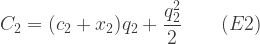
To illustrate these two interpretations of ‘best’ and how they can be achieved, let us flesh out our scenario with sufficient detail to permit the use of mathematical optimisation techniques. Let us assume that the government must pay the same unit price for all amounts of the good produced using a technique, but can discriminate in respect of price between the two techniques. Let the quantities produced using the two techniques be and . Suppose that each technique is available to many small firms with a range of production costs such that the aggregate production costs as progressively higher-cost firms come into production are (3):
Costs here are taken to include normal profit, so we can assume that a firm will produce if and only if the unit price offered by the government equals or exceeds its unit cost. At aggregate level, therefore, the quantity of the good produced by a technique will be such that the aggregate marginal cost (4) equals the price offered:
Suppose further that the government knows the above formulae and knows the values of and , but not of and . The latter, from the government’s point of view, are independent random variables, each with uniform distribution over the range where is a known constant. In the central case which we will consider the known values are: . We also assume that and .
To determine the unit price(s) the government should offer, it clearly needs to undertake some sort of auction process. I shall consider five possible types of auction, setting out the relevant maths in some detail for the first and in outline for the others (5).
An immediate question is whether the government should hold separate auctions for the two techniques or a single auction embracing both. I will consider the separate auctions (technology-specific) case first. This requires the government, using only the information it has, to determine the optimal quantities to be obtained by use of each technique. Because some of its information is stochastic, it needs to consider the expectation, denoted , of the range of possible outcomes of any choice of quantities, and choose the quantities that minimise that expectation.
If the aim is to minimise cost to the government, the problem can be formulated as:
Since we require , and using E3 and E4, we can eliminate and and express the problem as:
Given that the distributions of the variables and have been defined as symmetrical about zero, we have , so that on evaluating the expectation in E6 we can ignore the terms containing or . For future reference, we also note that, since and are independent, but and importantly are not zero but equal (6). Rearranging the terms not containing or , the problem becomes:
Differentiating with respect to , the first order condition is:
implying (7):
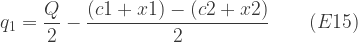
Substituting our known values we have = (20 – 100 + (2 x 100))/4 = 30, from which we can infer = 70, = 130 + , = 90 + . The implied expectation of the cost to the government is:
10,200
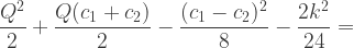
where, again, we can ignore terms containing or . Although the aim in this case was not to maximise welfare, we may note that the economic cost is:
Invite bids from technique 1, and set the strike price at the level just sufficient to bring forth production at the level ( = 30) determined by the minimum cost to government problem E5 AND Invite bids from technique 2, and set the strike price at the level just sufficient to bring forth production at the level ( = 70) determined by the problem E5.
It is important to note that this procedure (and all the others to be considered) only works because of our assumption that there are many small firms with a range of production costs. Because of this, we can take it that each firm’s bid reflects its actual costs. A firm can gain nothing from a higher bid since, with many small firms, such a bid cannot significantly raise the strike price, but can (if the bid exceeds the strike price) result in the firm losing the business it could have gained.
If the aim is to maximise welfare, which as we have seen requires minimising economic cost, the problem is formulated as:
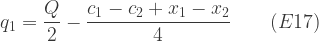
Substituting as before for and , eliminating terms in and , and setting the derivative with respect to equal to zero, we can obtain:
Substituting known values we have = 100/2 + 1.2(20 – 100) / 2.8 = 15.714. From this we can obtain the cost to the government (10,608) and the economic cost (9,054). As we might expect, the former is considerably more than when we aimed to minimise the cost to the government, while the latter is considerably less.
To obtain this outcome, we require Auction Type 2:
Invite bids from technique 1, and set the strike price at the level just sufficient to bring forth production at the level ( = 15.714) determined by the minimum economic cost problem E12 AND Invite bids from technique 2, and set the strike price at the level just sufficient to bring forth production at the level ( = 84.286) determined by the problem E12.
A feature of both the approaches we have considered is that, given our known values, they result in different prices for electricity according to the technique by which it is produced. Suppose instead that the government holds what we will call Auction Type 3:
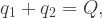
Invite bids from techniques 1 and 2, and set a single strike price at the level just sufficient to bring forth total production at the required level = 100).
In this case, from E3 and E4 we can infer:
implying:
Although we can infer formulae for and , these all contain the variables and . On calculating the expected cost to the government and drop out as before since we are simply multiplying the common price by the fixed quantity ; given our known values the expected cost to the government is 11,000. In calculating the expected economic cost, however, the production cost formulae include the squares of and resulting in squares of and which as we have seen take the expected value . The expected economic cost is 9,083, of which these expected values of squared variables contribute -102/6 = -17.
This type of auction does not achieve the best outcome on either of our interpretations of ‘best’. It results in an expected cost to the government higher than either Type 1 or Type 2, and an expected economic cost higher than Type 2. What it does minimise, by equalizing the prices and therefore the marginal costs of production using the two techniques, is the total production cost. But that is not what we want to minimize under either of our interpretations of ‘best’.
It may come as a surprise that the government can do better than any of the approaches considered so far. The key here is that the government can hold a single auction without committing itself to set a common strike price. This is sometimes termed a product mix auction (8), the principle being applicable to differentiated goods or to a common good that can be produced in more than one way. Given that, based on our assumptions, each firm’s bid reflects its actual costs, the set of bids received in an auction provides the government with a lot of cost information. It can use that information to choose strike prices for each technique according to its aim.
If the aim is to minimise the cost to the government, the problem to be solved after holding the auction is:
Proceeding as above, albeit without needing at this stage to consider the expectation, we obtain:
Note that we do not ignore the terms in and ; their values have effectively been revealed by the auction, so at this stage we are dealing with actual values, not with the expectation of a formula containing variables. Using E17 we can infer formulae for and , all of which contain and , and for the cost to the government for the particular values of and which is:
For purpose of comparison with our earlier results, especially from Auction Type 1, we want the expectation of E18 over the range of possible values of and , which is:
10,192
We can also calculate the expectation of the economic cost which is 9,326.
For this expected outcome we require Auction Type 4:
Invite bids from techniques 1 and 2, and using the results of the auction, set the strike prices for each technique at levels which a) are just sufficient to bring forth total production = 100 and b) among the combinations of strike prices which satisfy (a), minimise cost to the government.
If the aim is to minimise economic cost, the problem to be solved, again after holding the auction, is:
Proceeding as above, this can be solved to obtain:
The expected cost to the government is 10,604 and the expected economic cost is 9,037. These expected outcomes are achieved by Auction Type 5:
Invite bids from techniques 1 and 2, and using the results of the auction, set the strike prices for each technique at levels which a) are just sufficient to bring forth total production = 100 and b) among the combinations of strike prices which satisfy (a), minimise total economic costs.
Table 1 below summarises the above results.
Auction type
1
2
3
4
5
Minimising
Cost to govt
Economic cost
Cost of production
Cost to govt
Economic cost
No. of auctions
Separate auction for each technology
Single auction embracing both technologies
Pricing
Price for each technology
Common price
Price for each technology
Cost to govt
10,200
10,608
11,000
10,192
10,604
Economic cost
9,340
9,054
9,083
9,326
9,037
Table 1: Comparison of expected outcomes of auction types, assuming c1 = 100, c2 = 20, Q = 100, k = 10, λ = 0.2
What can be inferred from these results?
Firstly, the classification of auction types reveals an ambiguity in the term ‘technology-neutral’. Should we reserve that term for type 3 with a single auction and a single strike price? Or should we also include types 4 and 5, the product-mix auctions, on the grounds that they have a single auction embracing both technologies? The assertion is often made that climate change policies should be technology-neutral, often I suspect without awareness of the possibility of a product-mix auction.
Secondly, the choice of aim is important. Comparing auction types 1 and 4 on the one hand with types 2 and 5 on the other, the former result in the cost to government being c 400 (3.8%) lower, while the latter result in the economic cost being c 300 (3.2%) lower.
Thirdly, although the product-mix auctions 4 and 5 give the best results, the gains they offer relative to the best alternatives are very small, at least given the parameter values in our central case. Focusing on expected economic cost, type 5 yields an advantage of only 17 (0.2%) over type 2. Table 2 below shows the effects on expected economic cost of various changes in parameters, variation 0 being our central case. Variations 1-3 show that changes in have little effect on the advantage of type 5 over type 2, and variation 5 shows that a change in also has little effect. However, variations 4 and especially 6 show that larger values of , the half-width of the random variability in production cost, result in larger advantages of type 5 over type 2.
Auction type
2
3
5
Variation
0
c2 = 20; k = 10; λ = 0.2
9,054
9,083
9,037
1
c2 = 20; k = 10; λ = 0.1
7,987
7,983
7,970
2
c2 = 20; k = 10; λ = 0.0
6.900
6,883
6,883
3
c2 = 20; k = 10; λ = 0.4
11,158
11,283
11,140
4
c2 = 20; k = 18; λ = 0.2
9,054
9,046
8,999
5
c2 = 50; k = 10; λ = 0.2
11,857
11,858
11,840
6
c2 = 50; k = 40; λ = 0.2
11,857
11,608
11,583
Table 2: Effects of different parameter values on expected economic costs for selected auction types. All variations have c1 = 100 and Q = 100.
It can be seen that type 5 is superior to types 2 and 3 in all cases except variation 2, when with = 0 the expected economic costs with types 3 and 5 are equal. However, the advantage of type 5 over the better of types 2 and 3 is never more than 0.5% (variation 4).
Given that a product-mix auction may be perceived as introducing additional complexity for limited benefit, it is of interest to compare the outcomes of type 2, the technology-specific approach, and type 3, the technology-neutral common price approach. Looking at variations 0 and 4, and then at 5 and 6, it can be seen that, other things being equal, changes in do not affect the outcome of type 2, but do affect that of type 3 (because as we have seen of the squared terms in and ). As a consequence, increased variability in production cost (higher ) tends to favour type 3 over type 2, the difference in the case of variation 6 being 2.1%.
Comparing variations 0, 1, 2 and 3, it can be seen that the relative outcomes of types 2 and 3 are also affected by with higher values tending to favour type 2. However, only with = 0.4 in the case of variation 3 does the difference exceed 1%, and many empirical estimates of are considerably lower than that. Browning (1976) estimated its value for US taxes on labour income as in the range 0.09 to 0.16 (9). Harrison, Rutherford & Tarr (2002), in a study of Chile, found a value of 0.076 for VAT and 0.185 for a tariff (10). Auriol & Warlters (2009) found an average value across 38 African countries in the range 0.19 to 0.21 (11).
Conclusion
We have considered a limited range of scenarios. Alternative scenarios might include any or all of the following features: more than two available techniques; different production functions; larger firms with scope for gamesmanship; government providing subsidies rather than meeting full costs. The sorts of results we have obtained might not carry over to all scenarios.
However, it has been shown that, if a technology-neutral auction is taken to mean an auction with a common strike price for different techniques for producing the same good, it will not necessarily yield more economic welfare than a technology-specific auction. For the scenarios considered, however, the advantage of the technology-specific auction is very small given likely ratios of the excess burden of tax to the direct burden.
It has also been shown that a suitably designed product-mix auction, which can be considered technology-neutral in the sense that a single auction embraces alternative techniques, can achieve more economic welfare than any other auction type. However, the advantage over the best alternative auction type, in all the cases we have considered, is rather small.
Although the single auction common price approach is generally sub-optimal, from a welfare perspective it is no more than very slightly sub-optimal in any of the cases we have considered, except that in which the excess burden of tax ratio is very high. This suggests that a government aiming to maximise welfare may be unlikely to go far wrong with a technology-neutral approach.
Our most significant finding is a rather obvious one. Whether the auction type is technology-neutral or technology-specific, the choice of aim matters. An auction designed to minimise cost to the government will result in a sub-optimal outcome from a welfare perspective. Equally, an auction designed to maximise welfare will mean a higher cost than necessary to the government. The difference in both cases may be of the order of 3-4%.
For a more formal specification of the relation between firm-level and aggregate production costs see Fabra & Montero, as 2 above, p 6
Obtained by differentiating E1 and E2 with respect to q1 and q2 respectively.
Readers familiar with elementary algebra and calculus should be able, from the information given, to confirm all my results, although the algebra is in some cases rather tedious.
The long-delayed decision on the proposed West Cumbria Mining project in Cumbria, England, has been announced, to widespread criticism from the Climate Change Committee and others.
The BBC’s report of the decision and reactions is here. The analysis of the issues which I posted in March 2021, though slightly dated in a few respects, remains largely valid I believe.


 of the excess burden to the direct tax burden, and sometimes as the ratio of the sum of the excess and direct burdens to the direct burden, known as the marginal cost of public funds (MCF); thus MCF =
  .
. 
 . Suppose that each technique is available to many small firms with a range of production costs such that the aggregate production costs as progressively higher-cost firms come into production are (3):
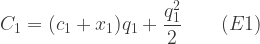


 and
and  , but not of
  and
and 
![[-k, k],](https://s0.wp.com/latex.php?latex=%5B-k%2C+k%5D%2C&bg=ffffff&fg=333333&s=1&c=20201002) where
where  is a known constant. In the central case which we will consider the known values are:
  . We also assume that
  and
and  .
.  , of the range of possible outcomes of any choice of quantities, and choose the quantities that minimise that expectation.
 ![\min E[p_1q_1+p_2q_2]\qquad(E5)](https://s0.wp.com/latex.php?latex=%5Cmin+E%5Bp_1q_1%2Bp_2q_2%5D%5Cqquad%28E5%29&bg=ffffff&fg=333333&s=1&c=20201002)
 , and using E3 and E4, we can eliminate
  and
and ![\min E[c_1+x_1+q_1)q_1+(c_2+x_2+Q-q_1)(Q-q_1)]\qquad(E6)](https://s0.wp.com/latex.php?latex=%5Cmin+E%5Bc_1%2Bx_1%2Bq_1%29q_1%2B%28c_2%2Bx_2%2BQ-q_1%29%28Q-q_1%29%5D%5Cqquad%28E6%29&bg=ffffff&fg=333333&s=1&c=20201002)
![E[x_1] = E[x_2] = 0,](https://s0.wp.com/latex.php?latex=E%5Bx_1%5D+%3D+E%5Bx_2%5D+%3D+0%2C&bg=ffffff&fg=333333&s=1&c=20201002) , so that on evaluating the expectation in E6 we can ignore the terms containing
, so that on evaluating the expectation in E6 we can ignore the terms containing ![E[x_1x_2] = E[x_1]E[x_2] = 0,](https://s0.wp.com/latex.php?latex=E%5Bx_1x_2%5D+%3D+E%5Bx_1%5DE%5Bx_2%5D+%3D+0%2C&bg=ffffff&fg=333333&s=1&c=20201002) but
but ![E[x_1^2],](https://s0.wp.com/latex.php?latex=E%5Bx_1%5E2%5D%2C&bg=ffffff&fg=333333&s=1&c=20201002) and
and ![E[x_2^2],](https://s0.wp.com/latex.php?latex=E%5Bx_2%5E2%5D%2C&bg=ffffff&fg=333333&s=1&c=20201002) importantly are not zero but equal
importantly are not zero but equal  (6). Rearranging the terms not containing
 ![\min [2q_1^2+(c_1-c_2-2Q)q_1 + c_2Q + Q^2]\qquad(E7)](https://s0.wp.com/latex.php?latex=%5Cmin+%5B2q_1%5E2%2B%28c_1-c_2-2Q%29q_1+%2B+c_2Q+%2B+Q%5E2%5D%5Cqquad%28E7%29&bg=ffffff&fg=333333&s=1&c=20201002)


 = 130 +
  = 90 +
 ![E[p_1q_1+p_2q_2]=E[(130+x_1)30+(90+x_2)70]=](https://s0.wp.com/latex.php?latex=E%5Bp_1q_1%2Bp_2q_2%5D%3DE%5B%28130%2Bx_1%2930%2B%2890%2Bx_2%2970%5D%3D&bg=ffffff&fg=333333&s=1&c=20201002) 10,200
10,200 
![E\Big[(c_1 + x_1)q_1 + \dfrac{q_1^2}{2} + (c_2 + x_2)q_2 + \dfrac{q_2^2}{2} + 10,200 \lambda \Big]](https://s0.wp.com/latex.php?latex=E%5CBig%5B%28c_1+%2B+x_1%29q_1+%2B+%5Cdfrac%7Bq_1%5E2%7D%7B2%7D+%2B+%28c_2+%2B+x_2%29q_2+%2B+%5Cdfrac%7Bq_2%5E2%7D%7B2%7D+%2B+10%2C200+%5Clambda+%5CBig%5D&bg=ffffff&fg=333333&s=1&c=20201002)
![= E\Big[(100 + x_1)30 + \dfrac{30^2}{2} + (20 + x_2)70 + \dfrac{70^2}{2} + 10,200(0.2)\Big]](https://s0.wp.com/latex.php?latex=%3D+E%5CBig%5B%28100+%2B+x_1%2930+%2B+%5Cdfrac%7B30%5E2%7D%7B2%7D+%2B+%2820+%2B+x_2%2970+%2B+%5Cdfrac%7B70%5E2%7D%7B2%7D+%2B+10%2C200%280.2%29%5CBig%5D&bg=ffffff&fg=333333&s=1&c=20201002) = 9,340
= 9,340 
![\min E\Big[(c_1 + x_1)q_1 + \dfrac{q_1^2}{2} + (c_2 + x_2)q_2 + \dfrac{q_2^2}{2} + \lambda (p_1q_1 + p_2q_2)\Big]\qquad(E12)](https://s0.wp.com/latex.php?latex=%5Cmin+E%5CBig%5B%28c_1+%2B+x_1%29q_1+%2B+%5Cdfrac%7Bq_1%5E2%7D%7B2%7D+%2B+%28c_2+%2B+x_2%29q_2+%2B+%5Cdfrac%7Bq_2%5E2%7D%7B2%7D+%2B+%5Clambda+%28p_1q_1+%2B+p_2q_2%29%5CBig%5D%5Cqquad%28E12%29&bg=ffffff&fg=333333&s=1&c=20201002)
 and
and 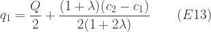
 = 100).
 and
and 

 10,192
![\min \Big[(c_1 + x_1)q_1 + \dfrac{q_1^2}{2} + (c_2 + x_2)q_2 + \dfrac{q_2^2}{2} + \lambda (p_1q_1 + p_2q_2)\Big]\qquad(E20)](https://s0.wp.com/latex.php?latex=%5Cmin+%5CBig%5B%28c_1+%2B+x_1%29q_1+%2B+%5Cdfrac%7Bq_1%5E2%7D%7B2%7D+%2B+%28c_2+%2B+x_2%29q_2+%2B+%5Cdfrac%7Bq_2%5E2%7D%7B2%7D+%2B+%5Clambda+%28p_1q_1+%2B+p_2q_2%29%5CBig%5D%5Cqquad%28E20%29&bg=ffffff&fg=333333&s=1&c=20201002)


